Something is wrong with realized volatility

If you own stocks of a company, how big is the risk to lose at least 5 percent of your money tomorrow? To answer that question, you need to know the variance of that stock. The problem with stock market variances is that they change a lot over time. They are very high in times of crises such as financial crises or political conflicts and they are far lower in calm times when uncertainty is low and the economy is doing well.

Due to these changes over time, we cannot just use the daily returns of the last year to estimate the volatility. This only gives us a long term average. So what can we do? The answer is to use realized volatility. The idea behind realized volatility is to increase the frequency of observation. Instead of using daily returns to estimate the yearly average, we use intraday returns to estimate the daily average.

These realized volatilities have pretty cool statistical properties. Unlike earlier econometric methods such as GARCH, realized volatility does not impose many assumptions on the way in which the volatility evolves over time. The important thing is only that the intraday stock returns are not correlated with each other. Since short term stock movements are largely unpredictable, the assumption about the uncorrelatedness of the returns does not seem to be much of a problem. In addition to that, we need the market to be very liquid so that we can use smaller and smaller intervals to calculate the realized volatility from.
If that is the case, then the estimated volatility is going to be reasonably close to the actual daily average volatility.

Due to these properties, realized volatility has become the standard for stock market volatility estimation over the last two decades. But there seems to be a problem. When you look at long term averages of realized variances and variances estimated from daily returns over the same time horizon the results do not lign up.

We looked at this issue in one of my last research papers. In theory, the variance of daily retuns and the average of the daily realized volatility should be the same if realized volatility really estimates the variance as it should.

Lets have a look what happens in practice.

library(tidyverse)
library(Hmisc)

First, we download realized volatility and stock market returns from the Oxford MAN Realized Library. The Realized Library is a project of the Oxford-Man Institute at the University of Oxford. It provides daily values for a number of variations of realized volatility for all major stock indices. The methods used are selected by Asger Lunde, Neil Shephard and Kevin Sheppard, who are some of the leading researchers in this field.

After reading in the latest zip-file, we calculate squared returns and rescale both the realized volatility and the squared return to annualized values.

# download latest data from the Oxford MAN Realized Library
data %>%
   mutate(sq_ret = data$open_to_close^2*252, 
             rv5 = rv5 * 252)

Note that we calculate the squared returns based on the return from market opening to market closing so that we omit the overnight return. This is done because the realized volatility typically also omits the overnight return. If we want the squared return to measure the same thing, we have to omit it, too.

data %>% glimpse()

## Observations: 142,134
## Variables: 21
## $ X1             2000-01-03, 2000-01-04, 2000-01-05, 2000-01-06, 2…
## $ Symbol         ".AEX", ".AEX", ".AEX", ".AEX", ".AEX", ".AEX", ".…
## $ open_time      90101, 90416, 90016, 90016, 90046, 90146, 90033, 9…
## $ medrv          4.978046e-05, 7.519469e-05, 1.663112e-04, 1.516630…
## $ open_to_close  -0.0003404608, -0.0336056730, -0.0016749893, -0.01…
## $ bv_ss          1.004276e-04, 2.070369e-04, 3.614080e-04, 2.582078…
## $ rv5            0.03280288, 0.05072902, 0.12372346, 0.05673518, 0.…
## $ bv             1.004276e-04, 2.070369e-04, 3.614080e-04, 2.582078…
## $ nobs           1795, 1785, 1801, 1799, 1798, 1794, 1795, 1797, 18…
## $ rv5_ss         1.301702e-04, 2.013057e-04, 4.909661e-04, 2.251396…
## $ close_time     163015, 163016, 163016, 163002, 163016, 163017, 17…
## $ rsv_ss         4.641401e-05, 1.469019e-04, 3.284684e-04, 1.160454…
## $ rv10           1.778898e-04, 2.605007e-04, 7.142078e-04, 1.818739…
## $ rk_parzen      1.789970e-04, 4.225273e-04, 3.240878e-04, 2.190503…
## $ close_price    675.44, 642.25, 632.31, 624.21, 644.86, 655.14, 64…
## $ rk_th2         1.016190e-04, 2.005050e-04, 3.447755e-04, 2.208909…
## $ rv10_ss        1.778898e-04, 2.605007e-04, 7.142078e-04, 1.818739…
## $ rk_twoscale    1.025169e-04, 1.987201e-04, 3.253867e-04, 2.180810…
## $ open_price     675.67, 664.20, 633.37, 632.46, 628.93, 651.82, 65…
## $ rsv            4.641401e-05, 1.469019e-04, 3.284684e-04, 1.160454…
## $ sq_ret         2.921022e-05, 2.845940e-01, 7.070085e-04, 4.344486…

Lets have a look at the squared return and the realized volatility. For ease of comparison, we take the log, so that the scale is not dominated by a few very large values.

data %>% 
  filter(Symbol == ".SPX") %>%
  mutate(time = X1) %>%
  select(time, rv5, sq_ret) %>%
  ggplot(aes(x=time)) +
  geom_line(aes(y=log(sq_ret))) +
  geom_line(aes(y=log(rv5)), col="red") +
  ggtitle("Log-realized volatility and log-squared return")

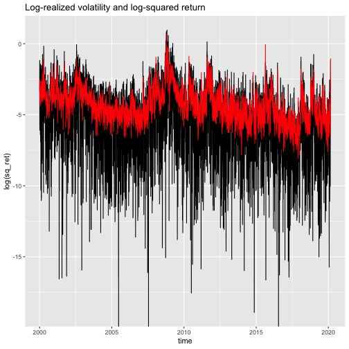
It is clear to see that both measures move together very closely, but the squared return in black fluctuates much more. This is because they both mesasure the same stock market variance, but the realized volatility has better statistical properties. It is a more precise estimator.

RV is biased

If both realized volatility and squared returns are ways to estimate the stock market volatility, then their long term averages should be the same. If we look at a longer timespan, the errors of the squared return that we see in the plot above should average out. So here is the test. It is taken from a paper that I wrote together with my co-author Janis Becker.

# calculate averages by index
tbl %>% 
          dplyr::select(Symbol, rv5, sq_ret) %>% 
            dplyr::group_by(Symbol) %>% 
              dplyr::summarise_all("mean")

# compare long term mean of realized volatility and squared returns
tbl %>%
  ggplot(aes(x=sq_ret, y=rv5)) +
    geom_text(aes(label=Symbol)) +
    geom_smooth(method='lm', se = FALSE) +
    geom_abline(slope=1, intercept=0)

In the first step we take the average of the realized variance and the squared return for every stock index in the Oxford MAN Realized Library. We then create a scatterplot with the mean squared return on the x-axis and the mean realized volatility on the y-axis. For comparison, we add the black 45 degree line. This is where the points would line up if the two means were actually the same. We also add a regression line (in blue) that describes how the relationship between the means really is in our dataset.

One can clearly see, that nearly all of the points are below the line. This means that the variance estimated using realized volatility is lower than the variance estimated using squared returns. The average deviation across all indices is 15 percent, which is also the deviation between the two means for the example of the S&P 500 index.

This is alarming! These variance estimates are used for risk management in financial institutions. If the variance is underestimated by 15 percent that means that all the risk measures calculated from them are off.

How do we know which one of the two means is off? Could the realized volatility be working fine and the squared returns are just a really bad estimator for the variance? Unfortunately, no. The squared return may be an imprecise estimator on a daily frequency, but we are looking at an average over 19 years here. With so many days to average over the law of large numbers can do its statistical magic and all the errors made on a daily basis will average out. When we use the squared return as an estimator for the variance, we do not make any assumptions about the returns or the dynamics of the variance that could not be correct. It works when the returns have a zero mean and that is an empirical fact.

The realized volatility on the other hand does make some assumptions on the dynamics of the volatility process and – even more importantly – about the dependence between intraday stock returns. These assumptions can be wrong. So the bias that we observe in the plot above must be due to a bias of the realized variance.

If you are familiar with the financial econometrics literature, you may say that it is well known that realized volatility can be biased due to market microstructure effects, so this is not a big deal. But then you are getting the size of this effect wrong.

An example of market microstructure effects is bid ask bounce. In the market there is offers to sell the stock for a certain ask price and offers to buy it for a certain bid price. The ask price is higher than the bid price. If a trade is initiated, somebody who wants to sell has to take the offer from somebody who wants to buy, or vice versa. Therefore some transactions are carried out at the bid price and some on the ask price. This causes prices to fluctuate a little bit, even though the value of the stock does not change.

If the stock we are looking at is relatively liquid so there are many transactions, these types of effects only start to play a role if we use intraday returns at a very high frequency (such as seconds) to calculate the realized volatility. Here we are looking at major stock indices, so liquidity should not be an issue, and the realized volatilities are calculated from 5-minute returns.

The academic literature broadly agrees that typical market microstructure effects do not play a role at this frequency. To dissolve any doubts in this direction even further we use 15 minute returns in the paper, and we use also realized volatility calculated using realized kernels – a technique to mitigate market microstructure effects. But nothing changes. Realized volatility has some kind of bias.

I am sure we are not the first people who have encountered this effect, but I am not aware that anybody has raised awareness for the fact that there is a bias that is so big and so consistent.

In the paper, we are trying to figure out where this effect could be coming from. We find that there seem to be some microstructure effects tied to calendar time that violate the assumptions of realized variance. If we omit the first and last half hour of the trading day, the effect disappears.

I am not a researcher anymore, so I hope that somebody will pick this topic up and pushes the research forward. A bias of this magnitude in realized volatility is too important to go overlooked.

If you are interested to find out more about our paper or if you are looking for a mathematically more precise description of the arguments and our attempts to explain this bias, you can find the paper here.